
From Resnet to ConvNeXt (Part 1): ResNet with Better Training Techniques
This is the first part of a series discussing and implementing (in PyTorch) the modernization process from a ResNet model to a ConvNeXt model, which was introduced in A ConvNet for the 2020s. The official repository is here.
In this part, we will discuss the context and motivation behind ConvNeXt, as well as the starting point of the modernization road map: good ‘ol ResNet, now with improved training techniques.
Context
Deep learning methods was not so attractive in the old days due to the lack of data and computational power. However, the last decade has been a time of rapid growth in deep learning research.
The use of convolutional neural networks (CNNs) in image processing has been studied for a long time, but has only really surged in popularity since 2012 after AlexNet1 achieved state-of-the-art performance in the ImageNet challenge. Another milestone moment for CNNs was in 2015, when the ResNet2 architecture was proposed. The residual learning scheme was introduced in the paper, and then became widely adopted in most if not all major CNNs architectures that followed.
Parallelly, the big moment for natural language processing (NLP) was the introduction of the Transformer3 architecture, which was introduced in 2018. The Transformer architecture was designed to be a general purpose NLP architecture that can be used for many tasks, including text summarization, translation, question answering, and more.
In 2020, reseachers at Google published a paper that describes an architecture that is Tranformer-based with minimal modification for the image recognition task, named Vision Transformer4 (ViT). It was shown that given sufficient data and model scale large enough, ViT can eventually outperform ResNets on many image classification datasets. However, one challenge was to apply ViT to other computer vision tasks, such as detection and segmentation. This was where hierarchical ViT came in. Hierarchical ViT like Swin Transformer5 (2021) with linear computation complexity to input image size can be used as a generic backbone for other vision tasks.
These historical developments ultimately led to our subject of discussion. In A ConvNet for the 2020s, the authors “gradually modernize a standard ResNet toward the design of a vision Transformer”.
The outcome of this exploration is a family of pure ConvNet models dubbed ConvNeXt. Constructed entirely from standard ConvNet modules, ConvNeXts compete favorably with Transformers in terms of accuracy and scalability, achieving 87.8% ImageNet top-1 accuracy and outperforming Swin Transformers on COCO detection and ADE20K segmentation, while maintaining the simplicity and efficiency of standard ConvNets.
The why of this paper is “to bridge the gap between the pre-ViT and post-ViT eras for ConvNets, as well as to test the limits of what a pure ConvNet can achieve”, driven by a key question:
How do design decisions in Transformers impact ConvNets’ performance?
ResNet: Architecture
Here is a quick refresher on the ResNet architecture.
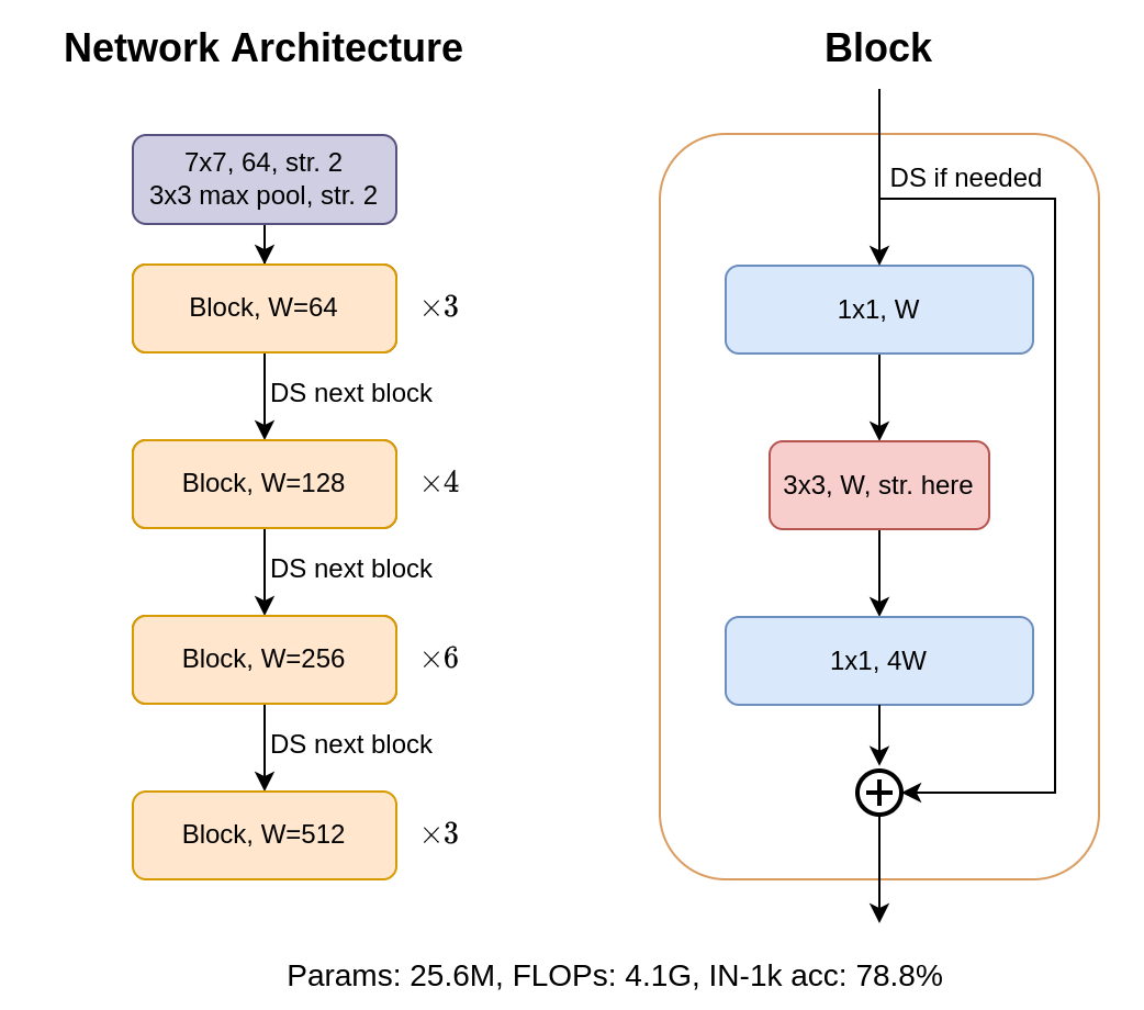
The above image describes a vanilla ResNet, specifically the ResNet-50 architecture. The key component here is the residual block, or Bottleneck block. The architecture itself is just repeated stacks of blocks with different specifications. Between each of the 4 stages illustrated in the left figure, the first block after each stage transition should downsample the input by a factor of 2 (convolution with stride 2). The stride is placed in the 3×3 conv. layer of that block. In the original paper, the stride is placed in the first 1×1 conv. layer. This difference actually gives the illustrated architecture the name ResNet1.5; this is also the default implementation in torchvision6 and was used as the baseline in the ConvNeXt paper.
Note that each convolution layer is followed by Batch Normalization7 and ReLU activation8. Also, the full architecture used for image classification also includes a pooling layer and a fully connected layer at the end.
ResNet: Implementation in PyTorch
Torchvision’s resnet.py is very flexible that similar architectures (ResNeXt, Wide-ResNet) can be easily created from the base by changing a few parameters. However, that comes with added redundant complexity and makes the code less readable, given that we only need vanilla ResNet. Thus we begin rewriting a simpler version of ResNet, start with importing stuffs and defining some helper functions, just to make the code more readable later.
from typing import Optional, Any, List
import torch.nn as nn
from torch import Tensor

def conv3x3(in_planes: int, out_planes: int, stride: int = 1) -> nn.Conv2d:
    return nn.Conv2d(in_planes, out_planes, kernel_size=3, stride=stride, padding=1, bias=False)

def conv1x1(in_planes: int, out_planes: int, stride: int = 1) -> nn.Conv2d:
    return nn.Conv2d(in_planes, out_planes, kernel_size=1, stride=stride, bias=False)

norm = nn.BatchNorm2d
relu = lambda : nn.ReLU(inplace=True)
I prefer to keep the type hinting :)
Bottleneck block
The implementation of the block is as follows:
class Block(nn.Module):
    expansion: int = 4

    def __init__(self, inplanes: int, width: int, stride: int = 1, projection: Optional[nn.Module] = None) -> None:
        super().__init__()
        self.relu = relu()
        self.projection = projection
        self.main_path = nn.Sequential(
            conv1x1(inplanes, width), norm(width), relu(),
            conv3x3(width, width, stride), norm(width), relu(),
            conv1x1(width, width * self.expansion), norm(width * self.expansion),
        )

    def forward(self, x: Tensor) -> Tensor:
        out = self.main_path(x)
        identity = x if self.projection is None else self.projection(x)
        out = self.relu(out + identity)
        return out
The expansion multiplier is fixed to 4.
Inside a block, in some cases the output and input can’t be directly added together due to dimension mismatch. Therefore, in such cases, we need to add a projection to the input shortcut path to match the output dimension. This is why Block takes a projection parameter, which is expected to be a nn.Module that transforms the input to match the output dimension.
In the next subsection, we will use 1×1 convolution and batch normalization for projection. Given knowledge of the architecture, we know we only need projection layers at the first block of each stage.
Also note that for ResNet-18 and ResNet-34, a simpler block structure with only two conv3x3 is used, called Basic block.
Constructing the model
Sequentially, in the code below we build the intial downsampling stem, the 4 stages, and the classifier (classification head). Each stage is created using a _make_stage function which we will define later.
class ResNet(nn.Module):
    def __init__(self, layers: List[int], num_classes: int = 1000) -> None:
        super().__init__()
        widths = [64, 128, 256, 512]
        self.inplanes = widths[0]
        # Downsampling stem downsamples input size by 4, e.g. 224 -> 56
        self.stem = nn.Sequential(
            # Assuming 3-channel input
            nn.Conv2d(3, widths[0], kernel_size=7, stride=2, padding=3, bias=False),
            norm(widths[0]),
            relu(),
            nn.MaxPool2d(kernel_size=3, stride=2, padding=1)
        )
        # Res1 -> Res4. No downsampling at the beginning of Res1.
        self.stages = nn.Sequential(
            *[self._make_stage(widths[i], layers[i], stride=2 if i != 0 else 1) for i in range(4)]
        )
        # Classification head
        self.head = nn.Sequential(
            nn.AdaptiveAvgPool2d((1, 1)),
            nn.Flatten(),
            nn.Linear(widths[-1] * Block.expansion, num_classes)
        )
        # Initialize weights
        self.apply(self._init_weights)

    def forward(self, x: Tensor) -> Tensor:
        x = self.stem(x)
        x = self.stages(x)
        x = self.head(x)
        return x
The base width is 64. The width is doubled after each stage ([64, 128, 256, 512]). Larger ResNets (e.g. ResNet-101, ResNet-200) are obtained by increasing stage depths rather than the base width.
We are missing two functions: _make_stage and _init_weights. The former is used to construct a stage, and the latter is used to initialize the weights. Both are pretty straightforward. For the _make_stage function, we just stack num_blocks blocks with width width together. The stride parameter is passed to the first block of the stage to downsample the input if needed. We also need projection layers for the first block. For weight initialization, we use He initialization9 for conv layers and init BN layers to have zero mean and unit variance:
    def _make_stage(self, width : int, num_blocks: int, stride: int = 1) -> nn.Sequential:
        blocks = []
        # Projection needed for first block of each stage
        projection = nn.Sequential(
            conv1x1(self.inplanes, width * Block.expansion, stride),
            norm(width * Block.expansion)
        )
        blocks.append(Block(self.inplanes, width, stride=stride, projection=projection))
        # Remaining blocks of the stage
        self.inplanes = width * Block.expansion
        for _ in range(1, num_blocks):
            blocks.append(Block(self.inplanes, width, stride=1, projection=None))
        return nn.Sequential(*blocks)

    def _init_weights(self, m: nn.Module) -> None:
        if isinstance(m, nn.Conv2d):
            nn.init.kaiming_normal_(m.weight, mode="fan_out")
        elif isinstance(m, nn.BatchNorm2d):
            nn.init.ones_(m.weight)
            nn.init.zeros_(m.bias)
        elif isinstance(m, nn.Linear):
            init_range = 1.0 / (m.out_features ** 0.5)
            nn.init.uniform_(m.weight, -init_range, init_range)
            nn.init.zeros_(m.bias)
Finally, to obtain various variants of ResNet:
def _resnet(layers: List[int], **kwargs: Any) -> ResNet:
    model = ResNet(layers, **kwargs)
    return model

def resnet50(**kwargs: Any) -> ResNet:
    return _resnet([3, 4, 6, 3], **kwargs)

def resnet101(**kwargs: Any) -> ResNet:
    return _resnet([3, 4, 23, 3], **kwargs)

def resnet200(**kwargs: Any) -> ResNet:
    return _resnet([3, 24, 36, 3], **kwargs)
Piece of cake, isn’t it :)
Improved training techniques
Training techniques
ResNet was introduced in 2015. Since then, better training techniques have been developed. In the paper, the authors adopted a training procedure similar to that of DeiT and Swin Transformer; and saw a substantial improvement in performance, e.g., from 76.1% to 78.8% on ImageNet for ResNet-50. The full hyperparameters table is in Appendix A.1 of the paper.
On ImageNet-1K, the batch size was set to 4096, and the number of epochs was 300. Such batch size is much larger, and the training time is longer than original ResNets’. The authors used AdamW optimizer10. Cosine learning rate decay was adopted, whereas in prior times, the learning rate had usually been either fixed; or decayed linearly/by step. They also used a warmup period of 20 epochs with linear growth to base learning rate.
Modern augmentation and regularization techniques were used. Nowadays, commonly used augmentations for pre-training and fine-tuning on image classification datasets include AutoAugment11/RandAugment12, Mixup13, CutMix14, etc. Detailed discussion on these techniques may be found in a future article :) Some techniques used solely for regularization include label smoothing, stochastic depth15, weight decay, and model EMA.
Stochastic depth integration
Unlike other augmentation and regularization techniques, stochastic depth needs to be integrated into the model at model definition time. We randomly drop a Res-block with probability \(p\), where \(p\) is a hyperparameter. In the simplest and also most widely used iteration of stochastic depth, \(p\) is the same for every block. More formally, let \(b \in \{0, 1\}\) be a Bernoulli random variable parameterized by \(p\); at training time, the output of each Res-block is:
\[H_l=ReLU(bf_l(H_{l-1}) + id_l(H_{l-1}))\]where \(f_l\) is the main forward path of block \(l\), \(id_l\) is the identity/projection function of block \(l\), and \(H_k\) denotes the output of layer \(k\).
We wrap our forward path in Block definition with a StochasticDepth module like this:
class Block(nn.Module):
    expansion: int = 4

    def __init__(
        self,
        inplanes: int,
        width: int,
        stride: int = 1,
        projection: Optional[nn.Module] = None,
        stodepth_survive: float = 1.
    ) -> None:
        super().__init__()
        self.relu = relu()
        self.projection = projection
        main_path = nn.Sequential(
            conv1x1(inplanes, width), norm(width), relu(),
            conv3x3(width, width, stride), norm(width), relu(),
            conv1x1(width, width * self.expansion), norm(width * self.expansion),
        )
        self.main_path = StochasticDepth(main_path, stodepth_survive) if stodepth_survive < 1. else main_path

    ...
Let us define our StochasticDepth class:
import torch

class StochasticDepth(nn.Module):
    """Randomly drop a module"""
    def __init__(self, module: nn.Module, survival_rate: float = 1.) -> None:
        super().__init__()
        self.module = module
        self.survival_rate = survival_rate
        self._drop = torch.distributions.Bernoulli(torch.tensor(1 - survival_rate))

    def forward(self, x: Tensor) -> Tensor:
        return 0 if self.training and self._drop.sample() else self.module(x)

    def __repr__(self) -> str:
        return self.module.__repr__() + f", stodepth_survival_rate={self.survival_rate:.2f}"
and add a parameter stodepth_survive to __init__ of ResNet. The final result can be found here:
Closing remarks
In this article, we have reviewed ResNet’s architecture and implementation, as well as a modern training recipe used in ConvNeXt. This will be the foundation for the next part of the series, where we will discuss and implement the modernizing roadmap from ResNet to ConvNeXt.