
From Resnet to ConvNeXt (Part 2): Modernizing a Vanilla ResNet
This is the second part of a series discussing and implementing (in PyTorch) the modernization process from a ResNet model to a ConvNeXt model, which was introduced in A ConvNet for the 2020s. The official repository is here.
In this part, we will gradually modify our ResNet base toward a ConvNeXt base, and see the contribution of each architecture change to the model’s performance.
Modernizing ResNet
We follow the modernizing roadmap in Section 2 of the paper, which consists of the following steps:
- Macro design
- ResNeXt-ify
- Inverted bottleneck
- Large kernel sizes
- Micro design
From now on, when we mention ResNet or model, either implicitly or explicitly, we will refer to ResNet-50 and the modified model from ResNet-50, if not otherwise specified.
Macro design
This part consists of 2 changes. The first change is to change the stage ratios. It is [3, 4, 6, 3] for ResNet-50, [3, 4, 23, 3] for ResNet-101, and [3, 24, 36, 3] for ResNet-200. The network grows deeper, but the base width remain the same that is 64.
Swin Transformer, on the other hand, uses a ratio of [1, 1, 3, 1] and [1, 1, 9, 1] for small and larger variants, respectively. Variants of Swin Transformer are obtained by using either of that two ratios and changing the base width. ConvNeXt adopts the same approach. We change the stage ratios to [3, 3, 9, 3]:
def resnet50(**kwargs: Any) -> ResNet:
    return _resnet([3, 3, 9, 3], **kwargs)
Technically, from this point forward it shouldn’t be called ResNet-50 anymore, but we will keep the name til the end :)
The second change is in the downsampling stem. ResNet uses a 7×7 convolution with stride 2, followed by a max-pooling with stride 2. Swin Transformer uses a “patchify” layer, which is a 4x4 non-overlapping convolution (stride 4) layer. We will use the same approach by modifying the stem:
### In ResNet.__init__()
self.stem = nn.Sequential(
    nn.Conv2d(3, self.inplanes, kernel_size=4, stride=4, bias=False),
    norm(self.inplanes),
)
The reported accuracy and FLOPs after these changes are 79.51% and 4.42G, respectively.
ResNeXt-ify
The core idea of ResNeXt1 is to use grouped convolution to reduce computional complexity: more groups equals less computation. By applying grouped convolution, we can increase other hyperparameters like the base width and model depths. We now change our 3×3 convolution layer in each block to depthwise separable convolution, which is a special case of grouped convolution, where the groups are the same as the number of channels. The idea of depthwise convolution is analogous to mixing information within each channel, that is “similar to the weighted sum operation in self-attention”.
### Helper function to replace conv3x3
def dwconv3x3(planes: int, stride: int = 1) -> nn.Conv2d:
    return nn.Conv2d(planes, planes, kernel_size=3, stride=stride, padding=1, groups=planes, bias=False)
### In Block.__init__()
main_path = nn.Sequential(
    conv1x1(inplanes, width), norm(width), relu(),
    dwconv3x3(width, stride), norm(width), relu(),
    conv1x1(width, width * self.expansion), norm(width * self.expansion),
)
The FLOPs massively reduced to 2.35G, as well as the reported accuracy; thus we increase the base width to 96. That also matches the widths of Swin-T.
### In ResNet.__init__()
widths = [96, 192, 384, 768]
The accuracy and FLOPs are now 80.5% and 5.27G, respectively.
Inverted bottleneck
The base block for building ResNet-50+ is called “Bottleneck”, because in order to reduce compution overhead for the 3×3 conv layer, it is sandwiched between two 1×1 convs, each responsible for temporary reducing and then expanding the number of channels, both by a factor of 4. This allows the network to grow deeper. However, as the field progresses, it is the inverted bottleneck architecture that is more widely used. It does the inverse of what the Bottleneck block does: it expands the number of channels by a factor of 4, do computation (3×3 conv) on the expanded planes, then reduces the channels by a factor of 4.
### In Block.__init__()
self.projection = projection

# Inverted bottleneck
expanded = width * self.expansion
main_path = nn.Sequential(
    conv1x1(inplanes, expanded), norm(expanded), relu(),
    dwconv3x3(expanded, stride), norm(expanded), relu(),
    conv1x1(expanded, width), norm(width),
)
The output dimension of each block is now width instead of width * Block.expansion. That means we have to change things in the model construction class as well. Firstly, the FC layer at the end should accept input dimension of widths[-1] instead of widths[-1] * Block.expansion. Secondly, now we need projection layers at the beginning block of stage 2, 3, 4 only instead of all 4. We also readjust the self.inplanes calculation in _make_stage():
### In ResNet.__init__()

# Classification head
self.head = nn.Sequential(
    nn.AdaptiveAvgPool2d((1, 1)),
    nn.Flatten(),
    nn.Linear(widths[-1], num_classes)
)
### ResNet._make_stage()

def _make_stage(self, width : int, num_blocks: int, stride: int = 1) -> nn.Sequential:
    blocks = []
    # Projection where needed
    projection = nn.Sequential(
        conv1x1(self.inplanes, width, stride),
        norm(width)
    ) if stride != 1 or self.inplanes != width else None
    blocks.append(
        Block(self.inplanes, width, stride=stride, projection=projection, stodepth_survive=self.stodepth)
    )
    # Remaining blocks of the stage
    self.inplanes = width
    for _ in range(1, num_blocks):
        blocks.append(Block(self.inplanes, width, stride=1, projection=None))
    return nn.Sequential(*blocks)
The reported accuracy and FLOPs are now 80.64% and 4.64G, respectively.
Large kernel
The popular standard for ConvNets is to stack many small-kernel convolutional layers. Swin Transformer performs self-attention within local windows with size of at least 7x7, which in some way is similar to the idea of large kernel convolution. Thus in the next step, authors explore the use of larger kernel for the depthwise convolution layer.
A prerequisites for this is to move the depthwise convolution layer up. The authors argued:
“That is a design decision also evident in Transformers: the MSA block is placed prior to the MLP layers. As we have an inverted bottleneck block, this is a natural design choice — the complex, inefficient modules (MSA, large-kernel conv) will have fewer channels, while the efficient, dense 1×1 layers will do the heavy lifting.”
### In Block.__init__()
expanded = width * self.expansion
main_path = nn.Sequential(
    dwconv3x3(inplanes, stride), norm(inplanes), relu(),
    conv1x1(inplanes, expanded), norm(expanded), relu(),
    conv1x1(expanded, width), norm(width),
)
The authors found that after the preparation steps, the benefit of adopting larger kernel-sized convolutions is now significant. The performance saturates at size 7×7, so we will replace the 3×3 depthwise convolution layer with a 7×7 correspondant.
### Helper function to replace dwconv3x3
def dwconv7x7(planes: int, stride: int = 1) -> nn.Conv2d:
    return nn.Conv2d(planes, planes, kernel_size=7, stride=stride, padding=3, groups=planes, bias=False)
### In Block.__init__()
expanded = width * self.expansion
main_path = nn.Sequential(
    dwconv7x7(inplanes, stride), norm(inplanes), relu(),
    conv1x1(inplanes, expanded), norm(expanded), relu(),
    conv1x1(expanded, width), norm(width),
)
The reported accuracy and FLOPs are now 80.57% and 4.15G, respectively.
Before the final, micro design changes, here is a checkpoint of the model architecture.
Micro design
The final modifications to the model consist of several small changes. Firstly, ReLU is replaced by GELU2; and BatchNorm is replaced by LayerNorm3. This also means we should bring back bias weight in the convolution layers, i.e. bias=True. Secondly, less norms and activations are used inside a block, such that a block would have the following structure:
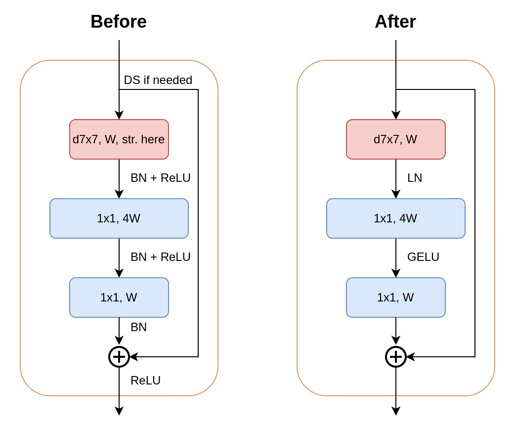
The figure on the left shows the architecture of a block after the “large kernel” step. The figure on the right shows the architecture of a block after the “micro design” step. Since we have reached the final steps, this is also the architecture of a ConvNeXt block.
We will soon run into trouble if we just replace nn.BatchNorm2d with nn.LayerNorm, because the our input (B, C, H, W) for nn.LayerNorm should be permuted to (B, H, W, C) for desired output; thus we create a sub-class of nn.LayerNorm for this:
class LayerNorm(nn.LayerNorm):
    """Permute the input tensor so that the channel dimension is the last one."""
    def __init__(self, num_features: int, eps: float = 1e-6, **kwargs: Any) -> None:
        super().__init__(num_features, eps=eps, **kwargs)

    def forward(self, x: Tensor) -> Tensor:
        return super().forward(x.permute(0, 2, 3, 1)).permute(0, 3, 1, 2)
This is not the most efficient implementation. In the official implementation, the authors use a neat trick: The 1×1 convolution is equivalent to a FC layer, thus we flatten and permute the output of 7×7dwconv and replace 1×1convs with FC layers. FC layers should be faster than 1x1 convolution. Normally we would not do this because the cost of permutating and flattening would outweight the benefit of implementing 1×1 conv with FC, but in this scenario since we need to permute the input anyway for nn.LayerNorm, the code should run slightly faster. Very cool :)
Our block definition should now be something like this:
### Helper function to replace norm and relu
norm = LayerNorm
gelu = lambda : nn.GELU()
class Block(nn.Module):
    expansion: int = 4

    def __init__(self, width: int, stodepth_survive: float = 1.) -> None:
        super().__init__()
        expanded = width * self.expansion
        main_path = nn.Sequential(
            dwconv7x7(width),
            norm(width),
            conv1x1(width, expanded),
            gelu(),
            conv1x1(expanded, width),
        )
        self.main_path = StochasticDepth(main_path, stodepth_survive) if stodepth_survive < 1. else main_path

    def forward(self, x: Tensor) -> Tensor:
        return x + self.main_path(x)
We see a massive reduction in code due to a single reason: we will use seperate downsampling layers between each stage. This change leads to:
- We no longer sometimes need a projection layer within a block.
- The input planes
inplanesis now identical towidth(because we can adjust it to match in the ds. layers), thus we remove the parameterinplanes. - We don’t need to use strided convolution within a block anymore.
Now more on the downsampling layers. In Swin Transformer, the spatial downsampling is achieved by a downsampling layer between each stage, contrary to our current approach where we perform downsampling at the first Res-block of each stage (except stage 1). We will use a non-overlapping 2×2 (stride 2) convolution layer to achieve this.
However, this leads to diverged training, and can be remedied by adding several LN layers where spatial resolution is reduced: before each downsampling layer, after the stem, and after the final global average pooling.
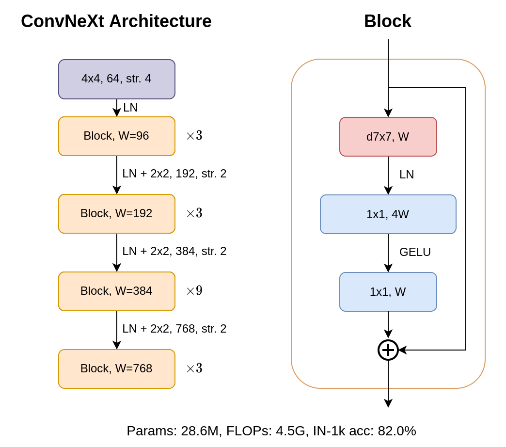
Finally, we have arrived at the final architecture. The smallest version of ConvNeXt, ConvNeXt-T, obtained from modernizing a ResNet-50, should have the following architecture:
class ResNet(nn.Module):
    def __init__(self, layers: List[int], num_classes: int = 1000, stodepth_survive: float = 1.) -> None:
        super().__init__()
        widths = [96, 192, 384, 768]
        self.inplanes = widths[0]
        self.stodepth = stodepth_survive
        # Downsampling stem downsamples input size by 4, e.g. 224 -> 56
        self.stem = nn.Sequential(
            nn.Conv2d(3, self.inplanes, kernel_size=4, stride=4),
            norm(self.inplanes),
        )
        # Stage 1 -> 4 and intermediate downsampling layers
        for idx, (layer, width) in enumerate(zip(layers, widths)):
            self.add_module(
                f"stage{idx + 1}",
                nn.Sequential(*[Block(width, stodepth_survive) for _ in range(layer)])
            )
            if idx == 3: break
            self.add_module(
                f"ds{idx + 1}",
                nn.Sequential(
                    norm(width),
                    nn.Conv2d(width, widths[idx + 1], kernel_size=2, stride=2),
                )
            )
        # Classification head
        self.head = nn.Sequential(
            nn.AdaptiveAvgPool2d((1, 1)),
            norm(widths[-1]),
            nn.Flatten(),
            nn.Linear(widths[-1], num_classes)
        )
        # Initialize weights
        self.apply(self._init_weights)
Creating a stage is now very simple, so we should remove the _make_stage function.
The forward pass should now take into account the intermediate downsampling layers:
    def forward(self, x: Tensor) -> Tensor:
        x = self.stem(x)

        x = self.stage1(x)
        x = self.ds1(x)
        x = self.stage2(x)
        x = self.ds2(x)
        x = self.stage3(x)
        x = self.ds3(x)
        x = self.stage4(x)

        x = self.head(x)
        return x
And we change _init_weights because now we use LayerNorm and we have brought back bias in convolution layers:
    def _init_weights(self, m: nn.Module) -> None:
        if isinstance(m, nn.Conv2d):
            nn.init.kaiming_normal_(m.weight, mode="fan_out")
            if m.bias is not None:
                nn.init.zeros_(m.bias)
        elif isinstance(m, nn.LayerNorm):
            nn.init.ones_(m.weight)
            nn.init.zeros_(m.bias)
        elif isinstance(m, nn.Linear):
            init_range = 1.0 / (m.out_features ** 0.5)
            nn.init.uniform_(m.weight, -init_range, init_range)
            nn.init.zeros_(m.bias)
And we have arrived at the final model. The accuracy on ImageNet-1k is 82.0%, and the FLOPs is around 4.5G!
ConvNeXt
The model we just obtained from modernizing the ResNet-50 architecture is dubbed ConvNeXt-T. Other variants of ConvNeXt are obtained by changing the stage ratios or the widths using the following specifications:
- ConvNeXt-T: C = (96, 192, 384, 768), B = (3, 3, 9, 3)
- ConvNeXt-S: C = (96, 192, 384, 768), B = (3, 3, 27, 3)
- ConvNeXt-B: C = (128, 256, 512, 1024), B = (3, 3, 27, 3)
- ConvNeXt-L: C = (192, 384, 768, 1536), B = (3, 3, 27, 3)
- ConvNeXt-XL: C = (256, 512, 1024, 2048), B = (3, 3, 27, 3)
where C is the widths of each stage, and B is the number of blocks in each stage.
We see that after each stage, the width grows by a factor of 2, and the ratios follow either the (1, 1, 3, 1) or (1, 1, 9, 1) pattern. Now we generalize our code to obtain the other variants of ConvNeXt by simply adding a base_width params to our model constructor. Also, it should be called ConvNext instead of ResNet now :)
class ConvNext(nn.Module):
    def __init__(self, base_width: int, layers: List[int], num_classes: int = 1000, stodepth_survive: float = 1.) -> None:
        super().__init__()
        widths = [base_width * (2**i) for i in range(4)]
        self.inplanes = widths[0] # Keep the same code as before
        ...
and to get the other variants:
def _convnext(base_width: int, layers: List[int], **kwargs: Any) -> ConvNext:
    model = ConvNext(base_width, layers, **kwargs)
    return model

def convnext_t(**kwargs: Any) -> ConvNext:
    return _convnext(96, [3, 3, 9, 3], **kwargs)

def convnext_s(**kwargs: Any) -> ConvNext:
    return _convnext(96, [3, 3, 27, 3], **kwargs)

def convnext_b(**kwargs: Any) -> ConvNext:
    return _convnext(128, [3, 3, 27, 3],**kwargs)

def convnext_l(**kwargs: Any) -> ConvNext:
    return _convnext(192, [3, 3, 27, 3], **kwargs)

def convnext_xl(**kwargs: Any) -> ConvNext:
    return _convnext(256, [3, 3, 27, 3], **kwargs)
The final code is here!
Closing remarks
In this article, we gradually modified the ResNet architecture to achieve ConvNeXt, following the roadmap of the original paper.
For the benchmarks, as well as ablation studies, great insights, and more discussion on the architecture, I encourage you to read the original paper and, of course, have a look at the official repository.
The thing I like about ConvNeXt is that the authors gave sensible reasons for the design decisions, either to pursue an pure ConvNet architecture that borrow “good” designs and traits of vision Transformers, or to adopt techniques in the ConvNet field that have been proven to work. The final result is a collective knowledge of years of research, as the authors said, “[the changes made] are not novel even in the ConvNet literature — they have all been researched separately, but not collectively, over the last decade”.
It is always great fun for me to try these things out, and I hope you enjoyed the series and learned something new from them!